Sunday’s conclusion to the 2016-17 EPL season produced an impressive haul of 37 goals. What’s more, they were all delivered in the space of 2 hours thanks to the final round of games being played simultaneously - truly the stuff dreams are made of for those watching at home.

Those 37 goals make this season’s finale the biggest scoring final round of fixtures in the 38-games-a-season era, but is this an all-time record? And how do final matchdays compare to the rest of the season - are they really the goalscoring extravaganzas they seem?

As in previous posts, let’s use engsoccerdata and the other usual suspects in R to answer these questions.

devtools::install_github("jalapic/engsoccerdata")
library(engsoccerdata)
require(dplyr)
require(ggplot2)

#update 'england' dataframe if there are new results
england <- rbind(england, subset(england_current(), !(Date %in% england$Date & home %in% england$home)))

#subset to PL era and prettify the season variable for plotting (e.g. '2016' -> '2016-17')
EPL <- subset(england, tier == 1 & Season %in% 1992:2016) %>%
  mutate(season = as.factor(paste0(Season, "-", substr(Season+1, 3, 4))))

Highest scoring final rounds

First thing to do is take a look at the number of goals scored in final rounds - that’s the last 10 games in seasons with 20 teams in the league and the last 11 games when there’s 22 teams.

lapply(unique(EPL$season), function(x) {
    #subset
    ss <- subset(EPL, season == x)
    #get number of games played in final round (i.e. 10 when 38 games a season, 11 when 42)
    GP <- n_distinct(ss$home) / 2
    #summarise
    ss %>%
      arrange(Date) %>%
      tail(GP) %>%
      summarise(season = as.factor(x), last.goals = sum(totgoal), GP)
}) %>%
plyr::rbind.fill() %>%
arrange(-last.goals)

##     season last.goals GP
## 1  1992-93         57 11
## 2  2016-17         37 10
## 3  2012-13         36 10
## 4  1994-95         35 11
## 5  2015-16         35 10
## 6  2007-08         34 10
## 7  1993-94         33 11
## 8  2000-01         32 10
## 9  2001-02         32 10
## 10 2009-10         32 10
## 11 2010-11         32 10
## 12 2011-12         32 10
## 13 2002-03         31 10
## 14 2004-05         30 10
## 15 1996-97         29 10
## 16 2003-04         29 10
## 17 2005-06         29 10
## 18 2006-07         29 10
## 19 2014-15         29 10
## 20 2013-14         28 10
## 21 1999-00         25 10
## 22 1998-99         24 10
## 23 1995-96         23 10
## 24 2008-09         23 10
## 25 1997-98         21 10

The final round of games in the 1992-93 season stands out on top with an astronomical 57 goals scored. Let’s have a look at those results:

EPL %>%
  arrange(Date) %>%
  subset(Season == 1992) %>%
  select(Date, home, visitor, FT) %>%
  tail(11)

##           Date                home             visitor  FT
## 452 1993-05-08       Coventry City        Leeds United 3-3
## 453 1993-05-08        Ipswich Town   Nottingham Forest 2-1
## 454 1993-05-08           Liverpool   Tottenham Hotspur 6-2
## 455 1993-05-08     Manchester City             Everton 2-5
## 456 1993-05-08       Middlesbrough        Norwich City 3-3
## 457 1993-05-08     Oldham Athletic         Southampton 4-3
## 458 1993-05-08    Sheffield United             Chelsea 4-2
## 459 1993-05-09 Queens Park Rangers         Aston Villa 2-1
## 460 1993-05-09           Wimbledon   Manchester United 1-2
## 461 1993-05-11             Arsenal   Tottenham Hotspur 1-3
## 462 1993-05-11 Queens Park Rangers Sheffield Wednesday 3-1

An 8-goal thriller, two 7-goal thrillers, three 6-goals games; in fact, not one team failed to score - must have been some Match Of The Day. (Watch this space for an incoming post on the best MotD ever, i.e. highest scoring days)

Now we might expect this number to be a bit higher as there were 11 games played per gameweek in that season, so let’s normalise the data to make these figures in terms of goals per game just to be fair.

lapply(unique(EPL$season), function(x) {
    #subset
    ss <- subset(EPL, season == x)
    #get number of games played in final round
    GP <- n_distinct(ss$home) / 2
    #summarise
    ss %>%
      arrange(Date) %>%
      tail(GP) %>%
      summarise(season = as.factor(x), last.goals.mean = round(sum(totgoal) / GP, 2))
}) %>%
  plyr::rbind.fill() %>%
  arrange(-last.goals.mean) %>%
  head(5)

##    season last.goals.mean
## 1 1992-93            5.18
## 2 2016-17            3.70
## 3 2012-13            3.60
## 4 2015-16            3.50
## 5 2007-08            3.40

It’s still far and away the highest scoring final round with 40% more goals per game than this season’s finale.

How does this compare to the all-time top-flight records, including the old First Division going all the way back to the 1888-89 season?

#subset all-time top flight
topflight <- subset(england, tier==1) %>%
  mutate(season = as.factor(paste0(Season, "-", substr(Season+1, 3, 4))))

lapply(unique(topflight$season), function(x) {
    #subset
    ss <- subset(topflight, season == x)
    #get number of games played in final round
    GP <- n_distinct(ss$home) / 2
    #summarise
    ss %>%
      arrange(Date) %>%
      tail(GP) %>%
      summarise(season = as.factor(x), total.goals = sum(totgoal), GP, goals.per.game = total.goals / GP)
}) %>%
  plyr::rbind.fill() %>%
  arrange(-total.goals) %>%
  head(5)

##    season total.goals GP goals.per.game
## 1 1992-93          57 11       5.181818
## 2 1960-61          54 11       4.909091
## 3 1931-32          48 11       4.363636
## 4 1961-62          48 11       4.363636
## 5 1963-64          48 11       4.363636

It stands as the all-time #1 (in terms of both total goals and goals per game), although I guess it would have been a less exciting Match of the Day as this final round of games was spread out over three days. Playing all 10 final fixtures simultaneously was only introduced in the 1994-95 season, making this Sunday the most goals scored in a final matchday.

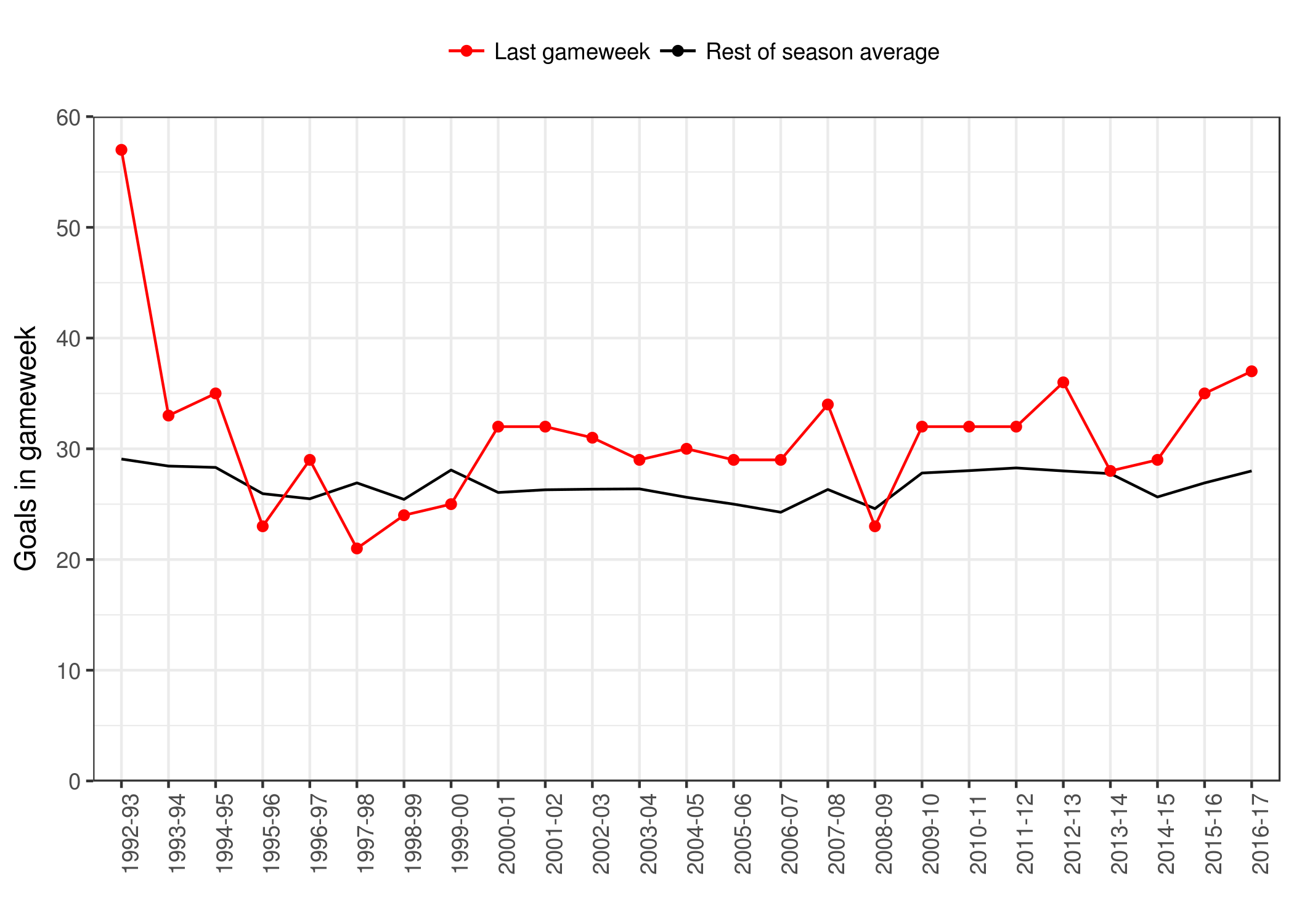
Let’s visualise this data to get a better feel for it, and calculate an average goals per gameweek from the rest of the season to compare each final round of fixtures to. The only fiddly thing is subsetting the final gameweek, as this can be 10 or 11 fixtures depending on the season (see footnote here). Code for all the plots can be found here.

d2 <- data.frame(
  #rest of season
  lapply(unique(EPL$Season), function(x) {
    #subset
    ss <- subset(EPL, Season == x)
    #get number of games played per round
    gpw <- n_distinct(ss$home) / 2
    #subset
    ss %>%
    arrange(Date) %>%
    tail(-gpw) %>%
    summarise(Season = x, rest.goals.mean = mean(totgoal) * gpw)
  }) %>%
  plyr::rbind.fill(),
  
  #final round of matches
  lapply(unique(EPL$Season), function(x) {
    #subset
    ss <- subset(EPL, Season == x)
    #get number of games in a gameweek
    gpw <- n_distinct(ss$home) / 2
    #subset
    ss %>%
    arrange(Date) %>%
    tail(gpw) %>%
    summarise(last.goals = sum(totgoal), gpw)
  }) %>%
  plyr::rbind.fill()
) %>%
#prettify season variable for plotting
mutate(season = as.factor(paste0(Season, "-", substr(Season+1, 3, 4))))

It would be nice to include some confidence intervals around our mean too, to get a better idea of just what constitutes a big-scoring gameweek for that season. The easiest way to do this was to split the season up into gameweeks, and calculate the mean and confidence intervals from that data (see footnote here).

#add gameweek variable
d3 <- lapply(unique(EPL$Season), function(x) {
  #subset by season
  EPL %>%
    subset(Season == x) %>%
    arrange(Date) %>%
    mutate(gameweek = rep(1:(n() / (n_distinct(home) / 2)), each = n_distinct(home) / 2) )
}) %>%
plyr::rbind.fill()

#split into 'last gameweek' and 'rest of season'
d4 <- data.frame(
  #last gameweek of season
  d3 %>%
    group_by(Season) %>%
    dplyr::filter(gameweek == max(gameweek)) %>%
    group_by(Season, gameweek) %>%
    summarise(matches = n(), goals = sum(totgoal)) %>%
    group_by(Season) %>%
    #sum goals and get number of fixtures per gameweek
    summarise(gpw = unique(matches), last.goals = goals) %>%
    select(last.goals, gpw),

  #rest of season
  d3 %>%
    group_by(Season) %>%
    dplyr::filter(gameweek != max(gameweek)) %>%
    group_by(Season, gameweek) %>%
    #get goals in each gameweek
    summarise(goals = sum(totgoal)) %>%
    group_by(Season) %>%
    #summmary statistics
    summarise(rest.goals.mean = mean(goals), rest.goals.sd = sd(goals), n.matches = n()) %>%
    mutate(rest.goals.se = rest.goals.sd / sqrt(n.matches), rest.goals.lower = rest.goals.mean - qt(1 - (0.05 / 2), n.matches - 1) * rest.goals.se, rest.goals.upper = rest.goals.mean + qt(1 - (0.05 / 2), n.matches - 1) * rest.goals.se) %>%
    select(Season, rest.goals.mean, rest.goals.lower, rest.goals.upper)
  ) %>%
  # prettify season variable again
  mutate(season = as.factor(paste0(Season, "-", substr(Season+1, 3, 4))))

Now we can re-draw the above figure with bands around the mean showing the 95% confidence interval.

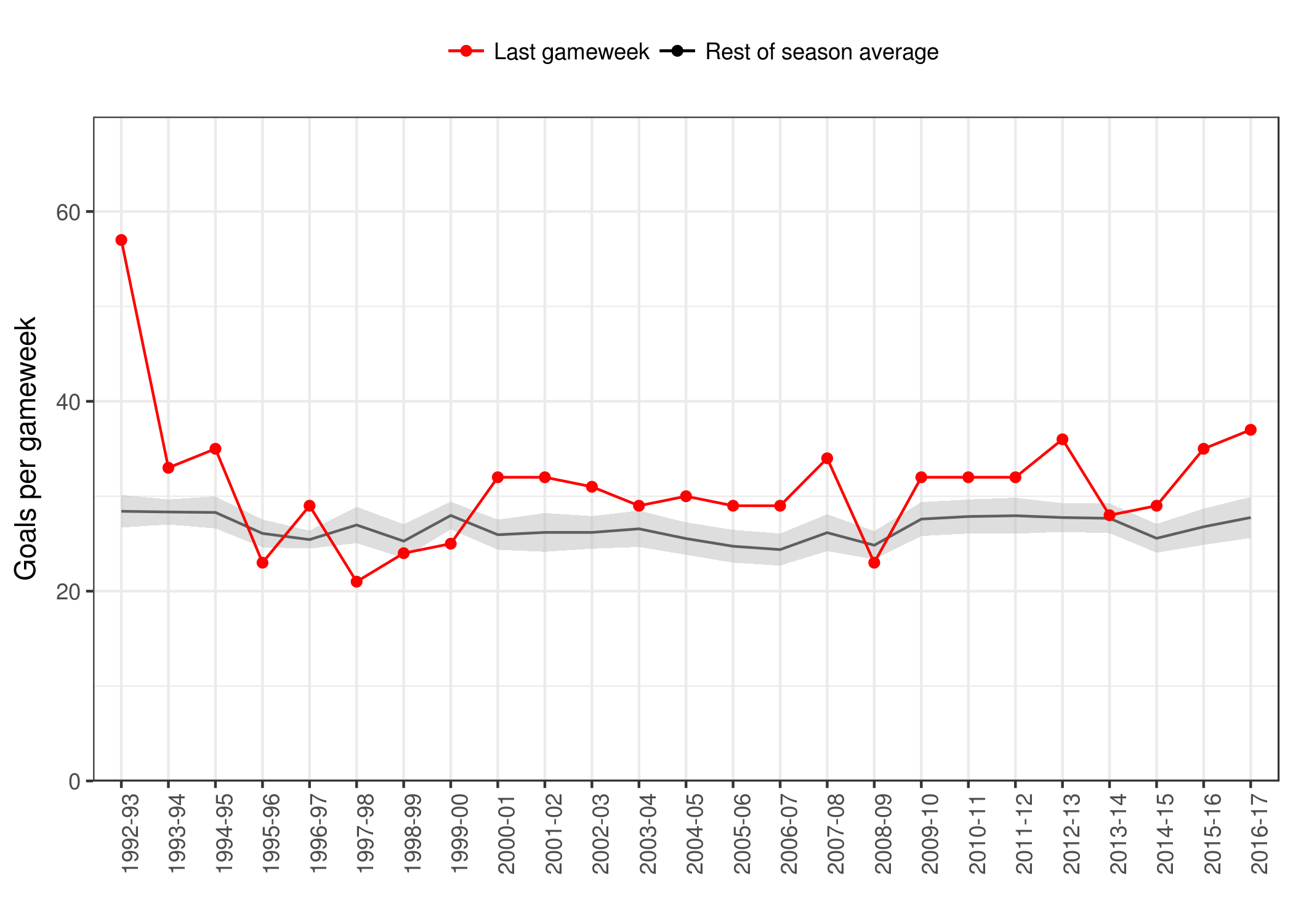
The rest of season average is slightly different in this second version (for this season, it’s now a mean of 37 different gameweek means, rather than a simple mean of 370 fixtures), but it seems like an acceptable estimate as it only differs by around 0.01 goals per game from our season-wide mean on average:

mean(abs(d2$rest.goals / d2$gpw) - (d4$rest.goals.mean / d4$gpw))

## [1] 0.01073003

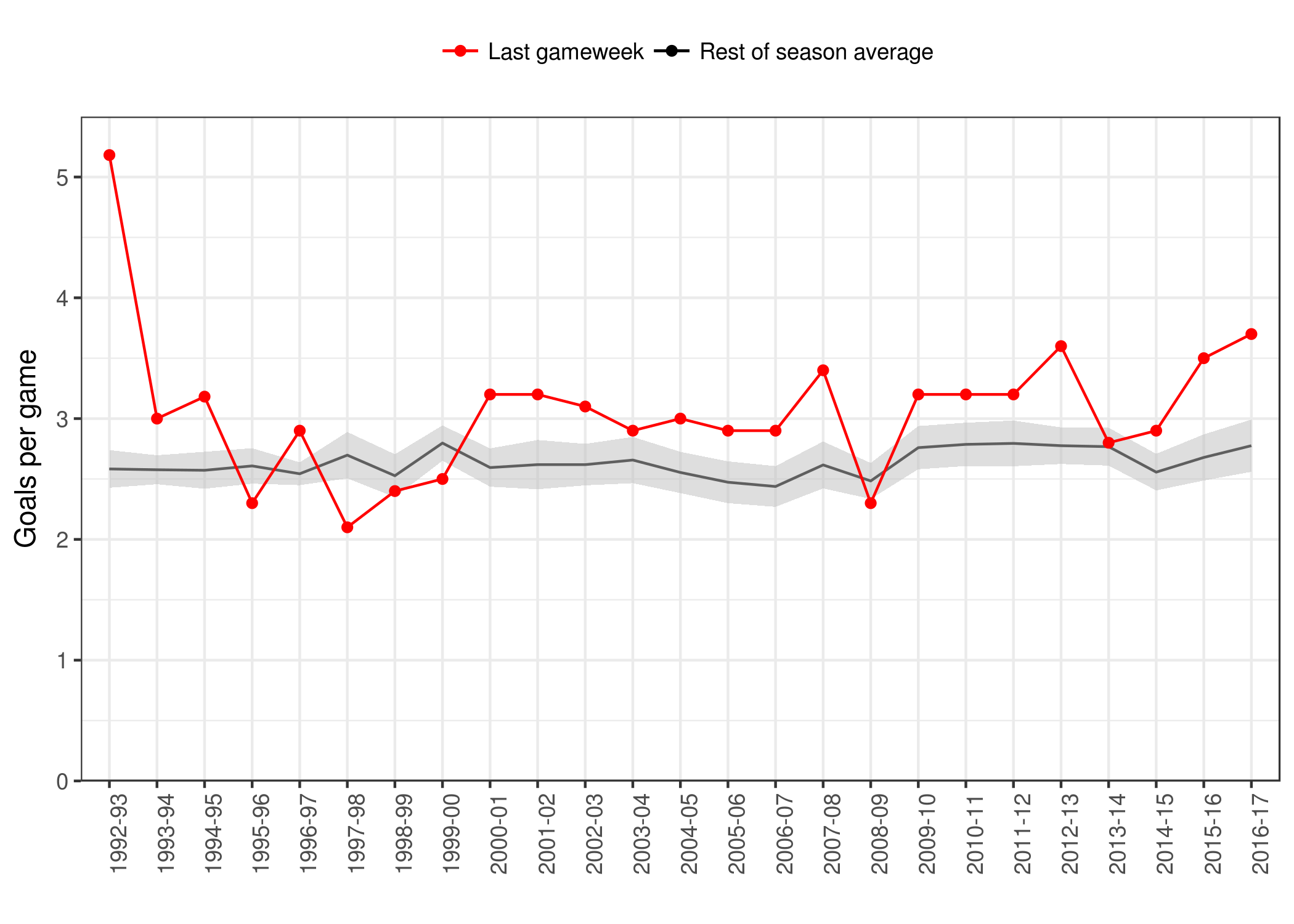
I like this second figure because total goals seems more intuitive than goals per game, but in the interests of fairness let’s plot the normalised goals per game data to account for the 11 games per gameweek in the first three PL seasons. It’s pretty much indistinguishable anyway.

Is the final round the highest scoring of the season?

So is it true that the last games of the season are always a goal rout?

nrow(subset(d2, last.goals > rest.goals.mean))

## [1] 20

Well, in 20 of the 25 Premier League seasons, the goals per game in the final round has been higher than the average. Although running the above functions across all 118 seasons of our topflight dataframe, the final gameweek was only higher than average 64 times; pretty much what we’d expect by random. Hmmm… Well how much higher are the PL finales?

mean(d2$last.goals / d2$rest.goals.mean)

## [1] 1.157592

We usually see around 15% more goals in the last PL gameweek than that season’s average gameweek. But how often is the last gameweek the highest scoring gameweek of the season?

d3 %>%
  group_by(Season, gameweek) %>% 
  summarise(goals = sum(totgoal)) %>%
  group_by(Season) %>%
  slice(which.max(goals)) %>%
  subset( (Season %in% 1992:1994 & gameweek == 42) | (Season %in% 1995:2016 & gameweek == 38) )

## Source: local data frame [1 x 3]
## Groups: Season [1]
## 
## # A tibble: 1 x 3
##   Season gameweek goals
##    <dbl>    <int> <int>
## 1   1992       42    57

Turns out only once: in that wild 1992-93 season finale. It’s not usually THE highest scoring, but where does the finale usually rank - 2nd highest, 3rd highest, etc…? Let’s have a look:

d3 %>%
  group_by(Season, gameweek) %>% 
  summarise(goals = sum(totgoal)) %>%
  group_by(Season) %>%
  mutate(rank = dense_rank(desc(goals))) %>%
  subset( (Season %in% 1992:1994 & gameweek == 42) | (Season %in% 1995:2016 & gameweek == 38) ) %>%
  select(Season, rank)

## Source: local data frame [25 x 2]
## Groups: Season [25]
## 
## # A tibble: 25 x 2
##    Season  rank
##     <dbl> <int>
##  1   1992     1
##  2   1993     4
##  3   1994     3
##  4   1995    11
##  5   1996     2
##  6   1997    13
##  7   1998     9
##  8   1999    11
##  9   2000     5
## 10   2001     5
## # ... with 15 more rows

If we take the median (middle) value as an average of these rankings, the final gameweek of the season is usually the 5th highest-scoring gameweek of the season. So usually not THE most exciting round but better than most.

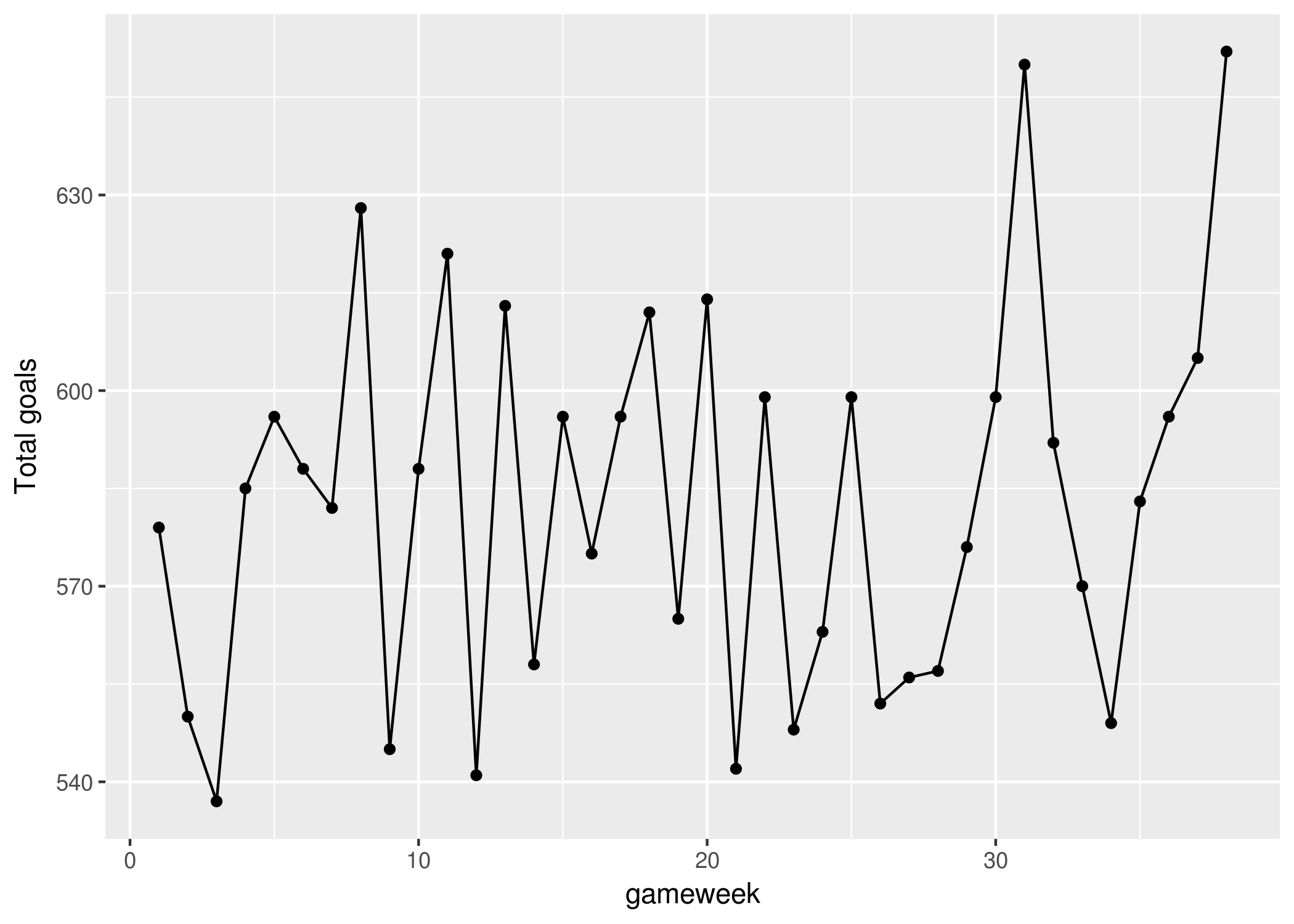
I’m disappointed by this apparent myth-busting and want some statistic to console me by telling me the final round is as exciting as I first suspected. So let’s have one final roll of the dice and just straight-up count how many goals have been scored in each of the 38 games weeks starting in 1994-95.

d4 <- subset(d3, ! Season %in% 1992:1994) %>%
  group_by(Season, gameweek) %>% 
  summarise(goals = sum(totgoal)) %>%
  group_by(gameweek) %>%
  summarise(goals = sum(goals)) %>%
  arrange(-goals)

There we go! Gameweek 38 has had the most. So together, I guess these stats tell us the season finale isn’t always the highest-scoring week of the season, but when it is, it more goals than any other gameweek.

I’m so happy to confirm my initial bias in some way that I’ll plot the data even though it doesn’t really need to be.

That’s it for this post. I’m still planning a short series of posts on ‘Robin Hood’ teams soon, but my next one will be a shorter one looking at most goals scored in a single day, a.k.a. the best Match Of The Day ever.

Footnote 1

There are unexpected anomalies that pop up when trying to manipulate any data. The one I didn’t expect in this data was when trying to get the number of games played in each gameweek, usually 10 or 11 depending on whether there were 20 or 22 teams in the league at the time. But then there was the bloody 1987-88 season, in which there were 21 teams in the league! I never knew this as it was before my time, but the First Division went through a bit of an awkward transition before reaching its modern 20-team form in 1995-96 season. The Football League decided to reduce the number of teams from 22 to 20 in the mid-80s, but did this over two seasons rather than in one fell swoop. A quirk of this transition was a relegation play-off at the end of 1987-88 season, which saw Chelsea as the first and only team to have been relegated from the top-flight through a play-off.

I wanted to see how they handled the fixture nightmare presented by having an odd-number of teams, and judging by engsoccerdata’s results archive, it seems the answer was badly. It looks bizzarely like Luton Town had to bear the brunt of this awkward season by playing 4 games in the space of 9 days - 2 of which being back-to-back games against Nottingham Forest:

topflight %>% 
  arrange(Date) %>% 
  subset(Season==1987) %>% 
  tail(11) %>%
  select(Date, home, visitor, FT)

##             Date                home           visitor  FT
## 36552 1988-05-07             Everton           Arsenal 1-2
## 36553 1988-05-07   Manchester United        Portsmouth 4-1
## 36554 1988-05-07    Newcastle United   West Ham United 2-1
## 36555 1988-05-07        Norwich City         Wimbledon 0-1
## 36556 1988-05-07   Nottingham Forest     Oxford United 5-3
## 36557 1988-05-07 Sheffield Wednesday         Liverpool 1-5
## 36558 1988-05-07         Southampton        Luton Town 1-1
## 36559 1988-05-09           Liverpool        Luton Town 1-1
## 36560 1988-05-09   Manchester United         Wimbledon 2-1
## 36561 1988-05-13          Luton Town Nottingham Forest 1-1
## 36562 1988-05-15   Nottingham Forest        Luton Town 1-1

But surely this can’t be true? I can’t find anything else online to confirm or refute this so if anyone has any information I’d love to know if this is right!

Footnote 2

Spitting the season into gameweeks was more troublesome than it first seemed due to rescheduled fixtures - for instance, one team’s 32nd game might take place in the same week as another team’s 33rd game. So I took some liberty by ordering each season’s results by date and splitting these results into an equal number of chunks (i.e. the number of gameweeks). This simplified method might mean that some gameweek chunks contain two games by the same teams whilst excluding other teams, but it’ll do for giving us some rough confidence intervals.