My last post looked at Robin Hood teams - taking points from the top teams only to give them away to the lower teams - and tried to quantify Hoodability as the difference in points per game (ppg) against the top 6 teams and ppg against the bottom 6.

However, this method has a couple of shortcomings. Firstly, by binning 20 league positions into two groups (top 6, bottom 6), we lose important information on performance against mid-table teams. Straight wins against the top 6 and defeats against positions 7th-15th is still at least a bit pertinent to Hoodability, isn’t it? Secondly, we have no real reason for comparing performance against the top 6 and the bottom 6; why not top 3 vs. bottom 3? Or top half vs. bottom half? We might do better with a measurement which treats league position as a continuous variable rather than splitting it into two discrete groups.

To address both these points, we’ll wrap up looking at Robin Hood teams by defining a more rigorous metric: comparing points per game with relative league position, i.e. how many points did a team get against an opposing side and how many places did that team finish above or below them in the league?

Let’s load the required packages to get our results data.

(Click here to show R code)

library(engsoccerdata)
library(dplyr)
library(ggplot2)
library(broom) #tidies output from lm models

# Update 'england' dataframe if there are new results
england <- rbind(england, subset(england_current(), tier == 1 & Season == 2016 & !(Date %in% england$Date & home %in% england$home)))

EPL <- subset(england, tier == 1 & Season %in% 1992:2016)

#set ggplot theme
my_theme <- theme_bw() +
  theme(
    axis.line = element_line(colour = "black"),
    axis.title = element_text(size=14, colour = "black"),
    axis.text = element_text(size=14, colour = "black"),
    legend.position = "none"
  )

First things first: let’s get the data on ppg against relative position for each team in each EPL season:

(Click here to show R code)

rel_pos <- lapply(1992:2016, function(x) {
  
  #make table for season
  xtab <- maketable_all(EPL, Season = x) %>%
    mutate(Pos = as.numeric(Pos)) %>%
    dplyr::select(team, Pos)
  
  #for each team
  lapply(xtab$team, function(y) {
    dd <- subset(homeaway(subset(EPL, Season==x)), team==y)
    dd <- merge(xtab, dd, by.x = "team", by.y = "team")
    dd$oppPos <- xtab$Pos[match(dd$opp, xtab$team)]
    dd$Pts <- ifelse(dd$gf > dd$ga, 3, ifelse(dd$gf < dd$ga, 0, 1))
    
    group_by(dd, oppPos) %>%
      summarise(Season = as.factor(Season[1]), team = team[1], Pos = Pos[1], dist = Pos[1] - oppPos[1], ppg = (mean(Pts))) %>% 
      select(-oppPos)
  }) %>%
  plyr::rbind.fill()
}) %>%
plyr::rbind.fill()

Now let’s get a feel for the data with some quick visualisations. First, ppg vs. relative league position across all teams and all seasons:

(Click here to show R code)

#relative league position vs. ppg
ggplot(rel_pos, aes(x = dist, y = ppg) ) + 
  geom_point(alpha=1/10) +
  # geom_jitter() +
  geom_smooth(method=lm) +
  xlab("Relative league position") +
  ylab("Points per game") +
  my_theme

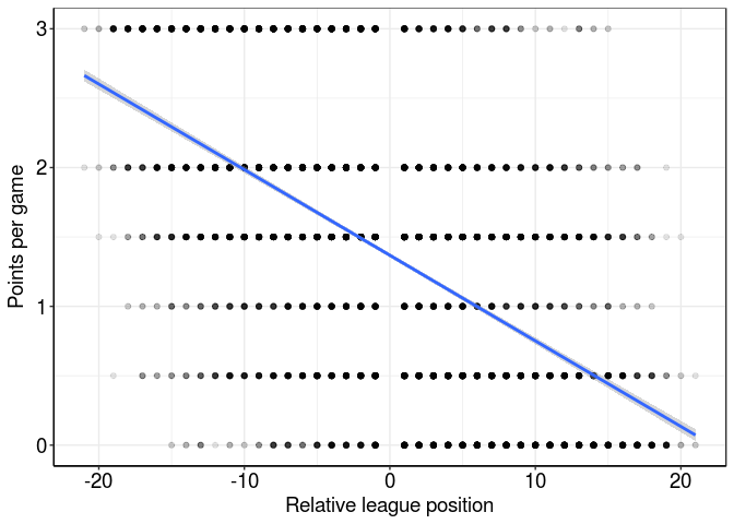
That’s a lot of overlapped points - even using transparency it’s hard to see how many points are at each point. We could do something fancy like 2D kernel density estimation to generate a heatmap:

(Click here to show R code)

ggplot(rel_pos, aes(dist, ppg)) + 
  stat_density2d(geom="tile", aes(fill = ..density..), n = 20, contour = FALSE) +
  scale_fill_gradient(low = "white", high = "red") +
  xlab("Relative league position") +
  ylab("Points per game") +
  my_theme

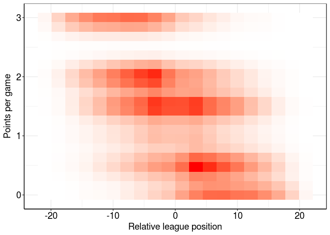
That might be a bit more helpful, but let’s simplify things even more by calculating mean ppg for each relative league position and plotting that:

(Click here to show R code)

# mean ppg for each relative league position
rel_pos2 <- group_by(rel_pos, dist) %>%
  summarise(ppg.mean = mean(ppg), ppg.se = plotrix::std.error(ppg))

#relative league position vs. mean ppg
ggplot(rel_pos2, aes(x = dist, y = ppg.mean) ) + 
  geom_point() +
  geom_smooth(method=lm) +
  xlab("Relative league position") +
  ylab("Points per game") +
  my_theme

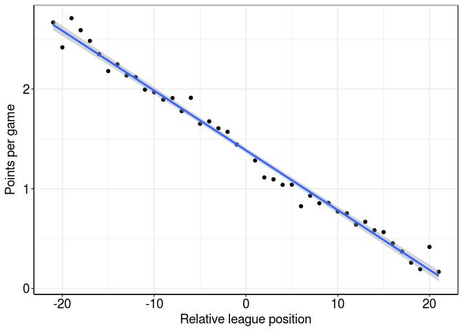
That’s as clear as day now: teams tend to get more points playing opposition teams that finish lower than them in the league. On average, a team can expect about 2 ppg against a team finishing 10 places below them and about 0.8 ppg against teams finishing 10 places above them. We can even see how many points each individual relative league position is worth by looking at the formula for the linear regression (which defines the blue line in the plot above).

#linear regression
lm(ppg.mean ~ dist, data=rel_pos2)

## 
## Call:
## lm(formula = ppg.mean ~ dist, data = rel_pos2)
## 
## Coefficients:
## (Intercept)         dist  
##     1.38496     -0.05992

So for each relative league position higher an opposing team is, we can expect to lose about -0.06 ppg (and gain 0.06 ppg for each relative league position lower the opposing team is).

But isn’t all this obvious? In fact, is it even possible for the slope of this line to be anything other than negative? After all, teams with a superior league position also have a superior ppg – isn’t that why they’re higher in the league?

Let’s investigate by looking at similar regression lines for individual teams.

A Robin Hood regression

We’ll start with Liverpool’s 2016-17 season, seeing as this was the focus of the previous post. Let’s draw this regression line (red) over the Premier League average (grey):

(Click here to show R code)

p <- ggplot(rel_pos2, aes(x = dist, y = ppg.mean) ) + 
  geom_smooth(method=lm, se=FALSE, col="grey") +
  geom_smooth(data=subset(rel_pos, team=="Liverpool" & Season==2016), aes(x = dist, y = ppg), method='lm', se=FALSE, col="red") +
  xlab("Relative league position") +
  ylab("Points per game") +
  my_theme
  
  p

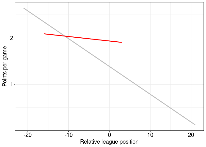
Ok, this line is a big flatter (less negative) than the league average. Let’s see how it compares with the extremes - the teams finishing first (Chelsea; blue) and last (Sunderland, dark red):

(Click here to show R code)

p + 
  geom_smooth(data=subset(rel_pos, team=="Chelsea" & Season==2016), aes(x = dist, y = ppg), method='lm', se=FALSE, col="blue") +
  geom_smooth(data=subset(rel_pos, team=="Sunderland" & Season==2016), aes(x = dist, y = ppg), method='lm', se=FALSE, col="darkred")

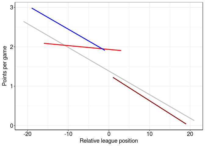
Chelsea sit pretty far above the line of best fit - probably because they had such a strong season, picking up 93 points. Sunderland are just below the line of best fit, perhaps indicating a particularly poor season. However, I’m more interested in the slope of these lines; the gradient of Chelsea and Sunderland’s lines looks pretty close to the average but Liverpool’s is much flatter. Perhaps we can compare use the coefficient of these slopes to define Hoodability?

Let’s start by getting regression coefficients for each team in the 2016-17 season.

(Click here to show R code)

# get regression coefficients
mods_2016 <- rel_pos %>%
  filter(Season==2016) %>%
  group_by(team) %>%
  do(fit = lm(ppg ~ dist, data = .)) %>%
  broom::tidy(fit) %>%
  subset(term=="dist") %>%
  select(team, estimate)
# get final league positions
xtab <- maketable_all(EPL, Season = 2016) %>%
  mutate(Pos = as.numeric(Pos)) %>%
  dplyr::select(team, Pos)
# join together
mods_2016 <- left_join(xtab, mods_2016, by = "team")

Reverse-ordering by slope, we can see Liverpool had the least negative slope of any team in the league last season:

(Click here to show R code)

mods_2016 %>%
  arrange(desc(estimate)) %>%
  head(5)

##             team Pos     estimate
## 1      Liverpool   4 -0.009669211
## 2      Hull City  18 -0.052345786
## 3 Crystal Palace  14 -0.052945924
## 4        Chelsea   1 -0.059649123
## 5 Leicester City  12 -0.065250199

And we can see this outlier by plotting slope vs. league position (Liverpool highlighted in red):

(Click here to show R code)

ggplot(mods_2016, aes(x = Pos, y = estimate)) +
  geom_point(size = 2) +
  geom_smooth(method = 'lm', col = "black") +
  geom_point(data=subset(mods_2016, team=="Liverpool"), aes(x = Pos, y = estimate), col="red", size = 2) +
  xlab("Final league position") +
  ylab("Slope of [ppg ~ relative position]") +
  my_theme

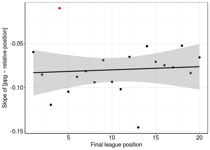
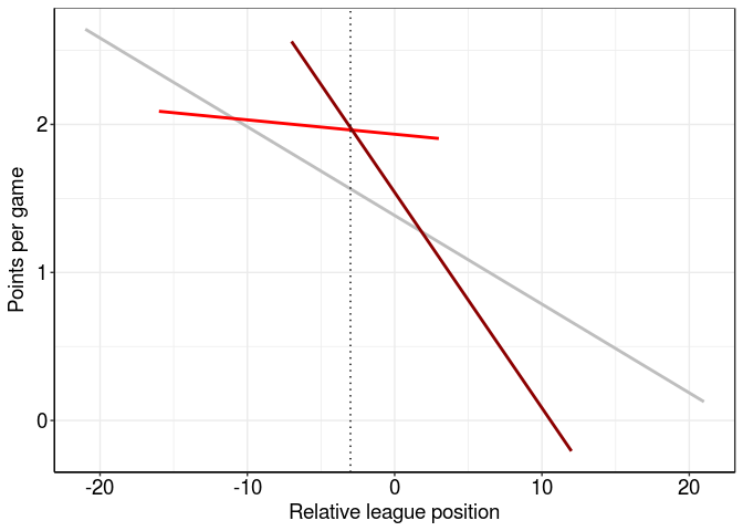
The other outlier - way below the line of best fit - is Stoke City. Their more-negative-than-average slope suggests they didn’t pick up many points against the top teams but were better at finishing off lower teams. In fact, plotting their individual slopes over the league average shows that Stoke (dark red) outperformed Liverpool (light red) against teams finishing more than two league places below them (dotted line at intercept, -2).

(Click here to show R code)

ggplot() + 
  geom_smooth(data = rel_pos2, aes(x = dist, y = ppg.mean), method=lm, se=FALSE, col="grey") +
  geom_smooth(data=subset(rel_pos, team=="Liverpool" & Season==2016), aes(x = dist, y = ppg), method='lm', se=FALSE, col="red") +
  geom_smooth(data=subset(rel_pos, team=="Stoke City" & Season==2016), aes(x = dist, y = ppg), method='lm', se=FALSE, col="darkred") +
  geom_vline(xintercept = -3, lty = 3) +
  xlab("Relative league position") +
  ylab("Points per game") +
  my_theme

But I digress; let’s calculate these regression coefficients for teams in every Premier League season. Then maybe we can find out the champion of our new Hoodability metric, and see whether there’s any relationship between Hoodability and performance.

Hoodability vs. performance

(Click here to show R code)

#get regression coefficients of teams for each season
mods_all <- lapply(unique(EPL$Season), function(x) {
  mods <- subset(rel_pos, Season==x) %>%
    group_by(team) %>%
    do(fit = lm(ppg ~ dist, data = .)) %>%
    broom::tidy(fit) %>%
    subset(term=="dist") %>%
    mutate(Season = x) %>%
    select(Season, team, estimate)
}) %>%
  plyr::rbind.fill() %>%
  arrange(desc(estimate))
# get final league positions for each season
x_tabs <- lapply(1992:2016, function(x) {
  maketable_all(EPL, Season = x) %>%
    mutate(Pos = as.numeric(Pos)) %>%
    mutate(Season = x) %>%
    dplyr::select(Season, team, Pos)
}) %>%
  plyr::rbind.fill()
# join together
mods_all <- left_join(mods_all, x_tabs, by = c("Season", "team"))

head(mods_all, 20)

##    Season                    team      estimate Pos
## 1    2002       Manchester United  0.0289473684   1
## 2    1992            Ipswich Town  0.0259504132  16
## 3    1993             Southampton  0.0244820559  18
## 4    1994            Ipswich Town  0.0233766234  22
## 5    1992           Middlesbrough  0.0209211318  21
## 6    1997          Leicester City  0.0202296120  10
## 7    2002        Blackburn Rovers  0.0164758790   6
## 8    2010 Wolverhampton Wanderers  0.0155640373  17
## 9    2006         West Ham United  0.0138184791  15
## 10   2010               Liverpool  0.0130008177   6
## 11   1992        Blackburn Rovers  0.0089872105   4
## 12   2000          Leicester City  0.0081135092  13
## 13   2013                 Chelsea  0.0060816681   3
## 14   1996          Leicester City  0.0031771247   9
## 15   2008           Middlesbrough  0.0031277927  19
## 16   1996                 Chelsea  0.0026982829   6
## 17   2000            Leeds United  0.0026293469   4
## 18   2010                 Everton  0.0022598870   7
## 19   2003         Manchester City  0.0004987531  16
## 20   2004         Birmingham City -0.0007942812  12

That’s 19 teams that have defied our naive logic by having a positive slope - that is, they picked up more points at higher teams than at lower teams. Seeing as this is probably as rigorous as I’m ever going to define Hoodability, I’ll go out on a limb and say these 19 teams are the true Robin Hoods of the Premier League, and that Man United are Robin Hood #1 in 2002-03 season - when they won the league.

We already seen them rank at #5 in our previous Hoodability metric last post, picking up 0.47 more ppg against the top 6 teams than against the bottom 6 (below). Looking at the rest of our new band of Merry Men, there’s some vindication for our previous method as most names are present in the figure below: Ipswich Town 1992-93 AND 1994-95, Southampton 1993-94, Leicester City 1997-98… But isn’t it nice to have spent all this time defining a more rigorous method to make sure though? ¹

Now we’ve got more data, we can plot Hoodability against final league position to see whether there’s any relationship with performance.

(Click here to show R code)

ggplot(mods_all, aes(x = Pos, y = estimate)) +
  geom_point(size = 2, alpha=0.8) +
  geom_smooth(method = 'lm', col = "black") +
  geom_hline(yintercept = 0, lty = 3) +
  xlab("Final league position") +
  ylab("Slope of [ppg ~ relative position]") +
  my_theme

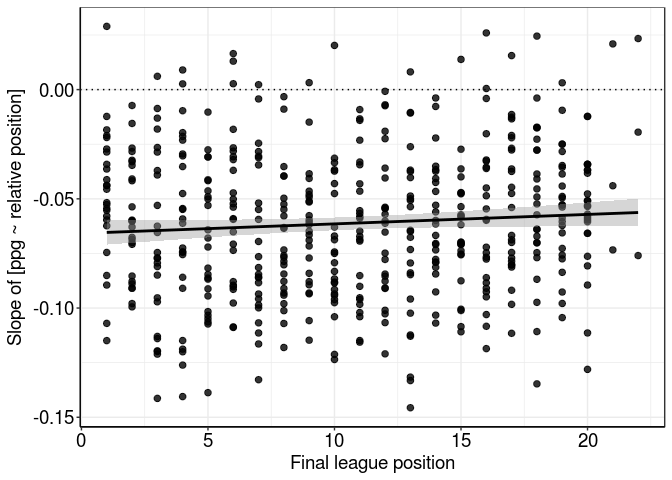
There might be the slightest positive relationship here, but I’m really not convinced there’s anything going on.. Not even statistical tests can discount common sense as a linear regression (yes, a regression fitted to regression coefficients) is not significant.

summary(lm(estimate ~ Pos, mods_all))

## 
## Call:
## lm(formula = estimate ~ Pos, data = mods_all)
## 
## Residuals:
##       Min        1Q    Median        3Q       Max 
## -0.085469 -0.023936 -0.000674  0.022927  0.094326 
## 
## Coefficients:
##               Estimate Std. Error t value Pr(>|t|)    
## (Intercept) -0.0658125  0.0030619 -21.494   <2e-16 ***
## Pos          0.0004337  0.0002523   1.719   0.0862 .  
## ---
## Signif. codes:  0 '***' 0.001 '**' 0.01 '*' 0.05 '.' 0.1 ' ' 1
## 
## Residual standard error: 0.03323 on 504 degrees of freedom
## Multiple R-squared:  0.00583,    Adjusted R-squared:  0.003857 
## F-statistic: 2.955 on 1 and 504 DF,  p-value: 0.08621

The decline of Robin Hood?

Finally, one last thing that I noticed quite at random. Let’s look at the average slope across all teams for each season in an animated plot using the gganimate package:

(Click here to show R code)

library(gganimate)
p <- ggplot(rel_pos, aes(x = dist, y = ppg, group = Season)) + 
  geom_smooth(aes(frame = as.numeric(Season)+1991, cumulative = TRUE), method=lm, se=FALSE, col="grey") +
  geom_smooth(aes(frame = as.numeric(Season)+1991), method=lm, se=FALSE, col="red") +
  xlab("Relative league position") +
  ylab("Points per game") +
  my_theme

gganimate(p, interval = c(rep(0.5, 24), 3), loop = TRUE)

Does it look like the slope is getting steeper over time, i.e. teams in more recent seasons show lower Hoodability? Let’s plot the slope coefficient for each season:

(Click here to show R code)

d <- lapply(unique(rel_pos$Season), function(x) {
ss <- subset(rel_pos, Season == x)
mod <- lm(ppg ~ dist, data = ss)
  data.frame(Season = x, slope = mod$coefficients[2])
  }) %>%
plyr::rbind.fill()

ggplot(d, aes(x = Season, y=slope)) +
  geom_point() +
  geom_smooth(aes(x = as.numeric(Season), y=slope), method=lm, col="black") +
  ylab("Slope of [ppg ~ relative position]") +
  xlab("") +
  my_theme +
  theme(axis.text.x = element_text(angle=90, hjust=1),
        legend.position = "top")

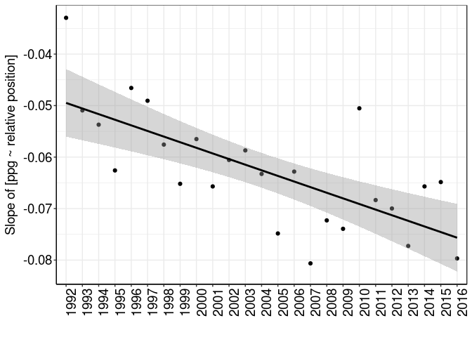
There definitely looks like a negative trend, but what does this mean? Teams are getting less Robin Hood-y in recent years, giving less points away to lower-placed teams relative to higher-placed teams? I’ve got no idea why this might be the case, though; thoughts on a postcard (or in the Discus comments below).

In conclusion…

That’s it for Robin Hood teams – I’m not sure how this idea spiralled into a two-part blog post so let’s never come back it again.

An interesting point was raised by a reader on the previous post as to what drives Hoodability - set pieces tend to account for a higher proportion of goals by lower-placed clubs, so perhaps clubs with high Hoodability are relatively poor at defending set pieces. There could certainly be some evidence for this idea looking at last season’s data:

I’ll be taking a closer look at the proportion of goals scored and conceded from set pieces over Premier League seasons and how this correlates with performance. I may also look at the effects of team height if I can get data for previous seasons; looking at last season, taller teams scored a higher proportion of their goals from set pieces - but also conceded a higher proportion from set pieces(!)